Compressed sensing using forward-backward

This tutorial presents a compressed sensing problem solved by the forward-backward splitting algorithm. The convex optimization problem is the sum of a data fidelity term and a regularization term which expresses a prior on the sparsity of the solution, given by

\[\min\limits_x \|Ax-y\|_2^2 + \tau \|x\|_1\]

where y are the measurements, A is the measurement matrix and \(\tau\) expresses the trade-off between the two terms.

The number of necessary measurements m is computed with respect to the signal size n and the sparsity level S in order to very often perform a perfect reconstruction. See [CR07] for details.

>>> n = 5000
>>> S = 100
>>> import numpy as np
>>> m = int(np.ceil(S * np.log(n)))
>>> print('Number of measurements: {}'.format(m))
Number of measurements: 852
>>> print('Compression ratio: {:3.2f}'.format(float(n) / m))
Compression ratio: 5.87

We generate a random measurement matrix A:

>>> np.random.seed(1)  # Reproducible results.
>>> A = np.random.normal(size=(m, n))

Create the S sparse signal x:

>>> x = np.zeros(n)
>>> I = np.random.permutation(n)
>>> x[I[0:S]] = np.random.normal(size=S)
>>> x = x / np.linalg.norm(x)

Generate the measured signal y:

>>> y = np.dot(A, x)

The prior objective to minimize is defined by

\[f_1(x) = \tau \|x\|_1\]

which can be expressed by the toolbox L1-norm function object. It can be instantiated as follows, while setting the regularization parameter tau:

>>> from pyunlocbox import functions
>>> tau = 1.0
>>> f1 = functions.norm_l1(lambda_=tau)

The fidelity objective to minimize is defined by

\[f_2(x) = \|Ax-y\|_2^2\]

which can be expressed by the toolbox L2-norm function object. It can be instantiated as follows:

>>> f2 = functions.norm_l2(y=y, A=A)

or alternatively as follows:

>>> f3 = functions.norm_l2(y=y)
>>> f3.A = lambda x: np.dot(A, x)
>>> f3.At = lambda x: np.dot(A.T, x)

Note

In this case the forward and adjoint operators were passed as functions not as matrices.

A third alternative would be to define the function object by hand:

>>> f4 = functions.func()
>>> f4._grad = lambda x: 2.0 * np.dot(A.T, np.dot(A, x) - y)
>>> f4._eval = lambda x: np.linalg.norm(np.dot(A, x) - y)**2

Note

The three alternatives to instantiate the function objects (f2, f3 and f4) are strictly equivalent and give the exact same results.

Now that the two function objects to minimize (the L1-norm and the L2-norm) are instantiated, we can instantiate the solver object. The step size for optimal convergence is \(\frac{1}{\beta}\) where \(\beta\) is the Lipschitz constant of the gradient of f2, f3, f4 given by:

\[\beta = 2 \cdot \|A\|_{\text{op}}^2 = 2 \cdot \lambda_{max} (A^*A).\]

To solve this problem, we use the Forward-Backward splitting algorithm which is instantiated as follows:

>>> step = 0.5 / np.linalg.norm(A, ord=2)**2
>>> from pyunlocbox import solvers
>>> solver = solvers.forward_backward(step=step)

Note

A complete description of the constructor parameters and default values is given by the solver object pyunlocbox.solvers.forward_backward reference documentation.

After the instantiations of the functions and solver objects, the setting of a starting point x0, the problem is solved by the toolbox solving function as follows:

>>> x0 = np.zeros(n)
>>> ret = solvers.solve([f1, f2], x0, solver, rtol=1e-4, maxit=300)
Solution found after 151 iterations:
    objective function f(sol) = 7.668167e+00
    stopping criterion: RTOL

Note

A complete description of the parameters, their default values and the returned values is given by the solving function pyunlocbox.solvers.solve() reference documentation.

Let’s display the results:

>>> import matplotlib.pyplot as plt
>>> _ = plt.figure()
>>> _ = plt.plot(x, 'o', label='Original')
>>> _ = plt.plot(ret['sol'], 'xr', label='Reconstructed')
>>> _ = plt.grid(True)
>>> _ = plt.title('Achieved reconstruction')
>>> _ = plt.legend(numpoints=1)
>>> _ = plt.xlabel('Signal dimension number')
>>> _ = plt.ylabel('Signal value')

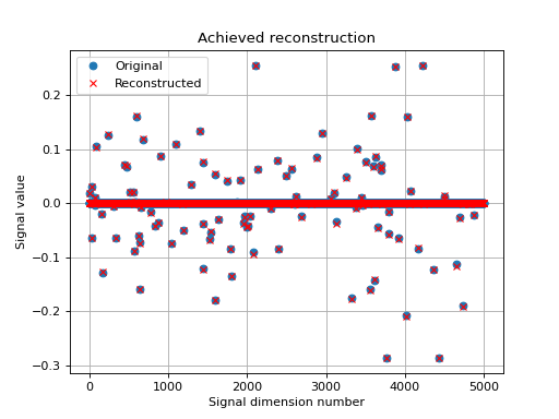
The above figure shows a good reconstruction which is both sparse (thanks to the L1-norm objective) and close to the measurements (thanks to the L2-norm objective).

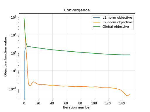
Let’s display the convergence of the two objective functions:

>>> objective = np.array(ret['objective'])
>>> _ = plt.figure()
>>> _ = plt.semilogy(objective[:, 0], label='L1-norm objective')
>>> _ = plt.semilogy(objective[:, 1], label='L2-norm objective')
>>> _ = plt.semilogy(np.sum(objective, axis=1), label='Global objective')
>>> _ = plt.grid(True)
>>> _ = plt.title('Convergence')
>>> _ = plt.legend()
>>> _ = plt.xlabel('Iteration number')
>>> _ = plt.ylabel('Objective function value')