Compressed sensing using Douglas-Rachford
This tutorial presents a compressed sensing problem solved by the Douglas-Rachford splitting algorithm. The convex optimization problem, a term which expresses a prior on the sparsity of the solution constrained by some data fidelity, is given by
where y are the measurements and A is the measurement matrix.
The number of necessary measurements m is computed with respect to the signal size n and the sparsity level S in order to very often perform a perfect reconstruction. See [CR07] for details.
>>> n = 900
>>> S = 45
>>> import numpy as np
>>> m = int(np.ceil(S * np.log(n)))
>>> print('Number of measurements: {}'.format(m))
Number of measurements: 307
>>> print('Compression ratio: {:3.2f}'.format(float(n) / m))
Compression ratio: 2.93
We generate a random measurement matrix A:
>>> np.random.seed(1)  # Reproducible results.
>>> A = np.random.normal(size=(m, n))
Create the S sparse signal x:
>>> x = np.zeros(n)
>>> I = np.random.permutation(n)
>>> x[I[0:S]] = np.random.normal(size=S)
>>> x = x / np.linalg.norm(x)
Generate the measured signal y:
>>> y = np.dot(A, x)
The first objective function to minimize is defined by
which can be expressed by the toolbox L1-norm function object. It can be instantiated as follows:
>>> from pyunlocbox import functions
>>> f1 = functions.norm_l1()
The second objective function to minimize is defined by
where \(\iota_C()\) is the indicator function of the set \(C = \left\{z \in \mathbb{R}^n \mid \|Az-y\|_2 \leq \epsilon \right\}\) which is zero if \(z\) is in the set and infinite otherwise. This function can be expressed by the toolbox L2-ball function object which can be instantiated as follows:
>>> f2 = functions.proj_b2(epsilon=1e-7, y=y, A=A, tight=False,
... nu=np.linalg.norm(A, ord=2)**2)
Now that the two function objects to minimize (the L1-norm and the L2-ball) are instantiated, we can instantiate the solver object. To solve this problem, we use the Douglas-Rachford splitting algorithm which is instantiated as follows:
>>> from pyunlocbox import solvers
>>> solver = solvers.douglas_rachford(step=1e-2)
After the instantiations of the functions and solver objects, the setting of a starting point x0, the problem is solved by the toolbox solving function as follows:
>>> x0 = np.zeros(n)
>>> ret = solvers.solve([f1, f2], x0, solver, rtol=1e-4, maxit=300)
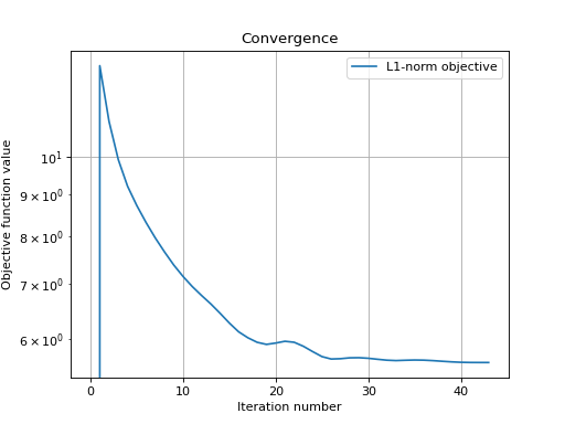
Solution found after 43 iterations:
objective function f(sol) = 5.607407e+00
stopping criterion: RTOL
Let’s display the results:
>>> import matplotlib.pyplot as plt
>>> _ = plt.figure()
>>> _ = plt.plot(x, 'o', label='Original')
>>> _ = plt.plot(ret['sol'], 'xr', label='Reconstructed')
>>> _ = plt.grid(True)
>>> _ = plt.title('Achieved reconstruction')
>>> _ = plt.legend(numpoints=1)
>>> _ = plt.xlabel('Signal dimension number')
>>> _ = plt.ylabel('Signal value')
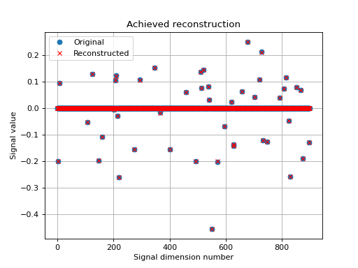
The above figure shows a good reconstruction which is both sparse (thanks to the L1-norm objective) and close to the measurements (thanks to the L2-ball constraint).
Let’s display the convergence of the objective function:
>>> objective = np.array(ret['objective'])
>>> _ = plt.figure()
>>> _ = plt.semilogy(objective[:, 0], label='L1-norm objective')
>>> _ = plt.grid(True)
>>> _ = plt.title('Convergence')
>>> _ = plt.legend()
>>> _ = plt.xlabel('Iteration number')
>>> _ = plt.ylabel('Objective function value')