Solvers
The pyunlocbox.solvers module implements a solving function (which will
minimize your objective function) as well as common solvers.
Solving
Call solve() to solve your convex optimization problem using your
instantiated solver and functions objects.
Interface
The solver base class defines a common interface to all solvers:
solver.pre(functions, x0) |
Solver-specific pre-processing. |
solver.algo(objective, niter) |
Call the solver iterative algorithm and the provided acceleration scheme. |
solver.post() |
Solver-specific post-processing. |
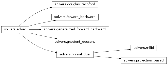
Solvers
Then, derived classes implement various common solvers.
gradient_descent(**kwargs) |
Gradient descent algorithm. |
forward_backward([accel]) |
Forward-backward proximal splitting algorithm. |
douglas_rachford([lambda_]) |
Douglas-Rachford proximal splitting algorithm. |
generalized_forward_backward([lambda_]) |
Generalized forward-backward proximal splitting algorithm. |
Primal-dual solvers (based on primal_dual)
mlfbf([L, Lt, d0]) |
Monotone+Lipschitz Forward-Backward-Forward primal-dual algorithm. |
projection_based([lambda_]) |
Projection-based primal-dual algorithm. |
-
pyunlocbox.solvers.solve(functions, x0, solver=None, atol=None, dtol=None, rtol=0.001, xtol=None, maxit=200, verbosity='LOW')[source]¶ Solve an optimization problem whose objective function is the sum of some convex functions.
This function minimizes the objective function \(f(x) = \sum\limits_{k=0}^{k=K} f_k(x)\), i.e. solves \(\operatorname{arg\,min}\limits_x f(x)\) for \(x \in \mathbb{R}^{n \times N}\) where \(n\) is the dimensionality of the data and \(N\) the number of independent problems. It returns a dictionary with the found solution and some informations about the algorithm execution.
Parameters: functions : list of objects
A list of convex functions to minimize. These are objects who must implement the
pyunlocbox.functions.func.eval()method. Thepyunlocbox.functions.func.grad()and / orpyunlocbox.functions.func.prox()methods are required by some solvers. Note also that some solvers can only handle two convex functions while others may handle more. Please refer to the documentation of the considered solver.x0 : array_like
Starting point of the algorithm, \(x_0 \in \mathbb{R}^{n \times N}\). Note that if you pass a numpy array it will be modified in place during execution to save memory. It will then contain the solution. Be careful to pass data of the type (int, float32, float64) you want your computations to use.
solver : solver class instance, optional
The solver algorithm. It is an object who must inherit from
pyunlocbox.solvers.solverand implement the_pre(),_algo()and_post()methods. If no solver object are provided, a standard one will be chosen given the number of convex function objects and their implemented methods.atol : float, optional
The absolute tolerance stopping criterion. The algorithm stops when \(f(x^t) < atol\) where \(f(x^t)\) is the objective function at iteration \(t\). Default is None.
dtol : float, optional
Stop when the objective function is stable enough, i.e. when \(\left|f(x^t) - f(x^{t-1})\right| < dtol\). Default is None.
rtol : float, optional
The relative tolerance stopping criterion. The algorithm stops when \(\left|\frac{ f(x^t) - f(x^{t-1}) }{ f(x^t) }\right| < rtol\). Default is \(10^{-3}\).
xtol : float, optional
Stop when the variable is stable enough, i.e. when \(\frac{\|x^t - x^{t-1}\|_2}{\sqrt{n N}} < xtol\). Note that additional memory will be used to store \(x^{t-1}\). Default is None.
maxit : int, optional
The maximum number of iterations. Default is 200.
verbosity : {‘NONE’, ‘LOW’, ‘HIGH’, ‘ALL’}, optional
The log level :
'NONE'for no log,'LOW'for resume at convergence,'HIGH'for info at all solving steps,'ALL'for all possible outputs, including at each steps of the proximal operators computation. Default is'LOW'.Returns: sol : ndarray
The problem solution.
solver : str
The used solver.
crit : {‘ATOL’, ‘DTOL’, ‘RTOL’, ‘XTOL’, ‘MAXIT’}
The used stopping criterion. See above for definitions.
niter : int
The number of iterations.
time : float
The execution time in seconds.
objective : ndarray
The successive evaluations of the objective function at each iteration.
Examples
>>> import numpy as np
>>> from pyunlocbox import functions, solvers
Define a problem:
>>> y = [4, 5, 6, 7]
>>> f = functions.norm_l2(y=y)
Solve it:
>>> x0 = np.zeros(len(y))
>>> ret = solvers.solve([f], x0, atol=1e-2, verbosity='ALL')
INFO: Dummy objective function added.
INFO: Selected solver: forward_backward
    norm_l2 evaluation: 1.260000e+02
    dummy evaluation: 0.000000e+00
INFO: Forward-backward method
Iteration 1 of forward_backward:
    norm_l2 evaluation: 1.400000e+01
    dummy evaluation: 0.000000e+00
    objective = 1.40e+01
Iteration 2 of forward_backward:
    norm_l2 evaluation: 2.963739e-01
    dummy evaluation: 0.000000e+00
    objective = 2.96e-01
Iteration 3 of forward_backward:
    norm_l2 evaluation: 7.902529e-02
    dummy evaluation: 0.000000e+00
    objective = 7.90e-02
Iteration 4 of forward_backward:
    norm_l2 evaluation: 5.752265e-02
    dummy evaluation: 0.000000e+00
    objective = 5.75e-02
Iteration 5 of forward_backward:
    norm_l2 evaluation: 5.142032e-03
    dummy evaluation: 0.000000e+00
    objective = 5.14e-03
Solution found after 5 iterations:
    objective function f(sol) = 5.142032e-03
    stopping criterion: ATOL
Verify the stopping criterion (should be smaller than atol=1e-2):
>>> np.linalg.norm(ret['sol'] - y)**2
0.00514203...
Show the solution (should be close to y w.r.t. the L2-norm measure):
>>> ret['sol']
array([ 4.02555301,  5.03194126,  6.03832952,  7.04471777])
Show the used solver:
>>> ret['solver']
'forward_backward'
Show some information about the convergence:
>>> ret['crit']
'ATOL'
>>> ret['niter']
5
>>> ret['time']
0.0012578964233398438
>>> ret['objective']
[[126.0, 0], [13.99999999..., 0], [0.29637392..., 0], [0.07902528..., 0],
[0.05752265..., 0], [0.00514203..., 0]]
-
class
pyunlocbox.solvers.solver(step=1.0, accel=None)[source]¶ Bases:
objectDefines the solver object interface.
This class defines the interface of a solver object intended to be passed to the
pyunlocbox.solvers.solve()solving function. It is intended to be a base class for standard solvers which will implement the required methods. It can also be instantiated by user code and dynamically modified for rapid testing. This class also defines the generic attributes of all solver objects.Parameters: step : float
The gradient-descent step-size. This parameter is bounded by 0 and \(\frac{2}{\beta}\) where \(\beta\) is the Lipschitz constant of the gradient of the smooth function (or a sum of smooth functions). Default is 1.
accel : pyunlocbox.acceleration.accel
User-defined object used to adaptively change the current step size and solution while the algorithm is running. Default is a dummy object that returns unchanged values.
-
pre(functions, x0)[source]¶ Solver-specific pre-processing. See parameters documentation in
pyunlocbox.solvers.solve()documentation.Notes
When preprocessing the functions, the solver should split them into two lists: * self.smooth_funs, for functions involved in gradient steps. * self.non_smooth_funs, for functions involved proximal steps. This way, any method that takes in the solver as argument, such as the methods in
pyunlocbox.acceleration.accel, can have some context as to how the solver is using the functions.
-
algo(objective, niter)[source]¶ Call the solver iterative algorithm and the provided acceleration scheme. See parameters documentation in
pyunlocbox.solvers.solve()Notes
The method
self.accel.update_sol()is called beforeself._algo()because the acceleration schemes usually involves some sort of averaging of previous solutions, which can add some unwanted artifacts on the output solution. With this ordering, we guarantee that the output of solver.algo is not corrupted by the acceleration scheme.Similarly, the method
self.accel.update_step()is called afterself._algo()to allow the step update procedure to act directly on the solution output by the underlying algorithm, and not on the intermediate solution output by the acceleration scheme inself.accel.update_sol().
-
post()[source]¶ Solver-specific post-processing. Mainly used to delete references added during initialization so that the garbage collector can free the memory. See parameters documentation in
pyunlocbox.solvers.solve().
-
-
class
pyunlocbox.solvers.gradient_descent(**kwargs)[source]¶ Bases:
pyunlocbox.solvers.solverGradient descent algorithm.
This algorithm solves optimization problems composed of the sum of any number of smooth functions.
See generic attributes descriptions of the
pyunlocbox.solvers.solverbase class.Notes
This algorithm requires each function implement the
pyunlocbox.functions.func.grad()method.See
pyunlocbox.acceleration.regularized_nonlinearfor a very efficient acceleration scheme for this method.Examples
>>> import numpy as np
>>> from pyunlocbox import functions, solvers
>>> dim = 25;
>>> np.random.seed(0)
>>> xstar = np.random.rand(dim) # True solution
>>> x0 = np.random.rand(dim)
>>> x0 = xstar + 5.*(x0 - xstar) / np.linalg.norm(x0 - xstar)
>>> A = np.random.rand(dim, dim)
>>> step = 1/np.linalg.norm(np.dot(A.T, A))
>>> f = functions.norm_l2(lambda_=0.5, A=A, y=np.dot(A, xstar))
>>> fd = functions.dummy()
>>> solver = solvers.gradient_descent(step=step)
>>> params = {'rtol':0, 'maxit':14000, 'verbosity':'NONE'}
>>> ret = solvers.solve([f, fd], x0, solver, **params)
>>> pctdiff = 100*np.sum((xstar - ret['sol'])**2)/np.sum(xstar**2)
>>> print('Difference: {0:.1f}%'.format(pctdiff))
Difference: 1.3%
-
class
pyunlocbox.solvers.forward_backward(accel=<pyunlocbox.acceleration.fista object>, **kwargs)[source]¶ Bases:
pyunlocbox.solvers.solverForward-backward proximal splitting algorithm.
This algorithm solves convex optimization problems composed of the sum of a smooth and a non-smooth function.
See generic attributes descriptions of the
pyunlocbox.solvers.solverbase class.Parameters: accel :
pyunlocbox.acceleration.accelAcceleration scheme to use. Default is
pyunlocbox.acceleration.fista(), which corresponds to the ‘FISTA’ solver. Passingpyunlocbox.acceleration.dummy()instead results in the ISTA solver. Note that while FISTA is much more time-efficient, it is less memory-efficient.Notes
This algorithm requires one function to implement the
pyunlocbox.functions.func.prox()method and the other one to implement thepyunlocbox.functions.func.grad()method.See [BT09a] for details about the algorithm.
Examples
>>> import numpy as np
>>> from pyunlocbox import functions, solvers
>>> y = [4, 5, 6, 7]
>>> x0 = np.zeros(len(y))
>>> f1 = functions.norm_l2(y=y)
>>> f2 = functions.dummy()
>>> solver = solvers.forward_backward(step=0.5)
>>> ret = solvers.solve([f1, f2], x0, solver, atol=1e-5)
Solution found after 15 iterations:
    objective function f(sol) = 4.957288e-07
    stopping criterion: ATOL
>>> ret['sol']
array([ 4.0002509 ,  5.00031362,  6.00037635,  7.00043907])
-
class
pyunlocbox.solvers.generalized_forward_backward(lambda_=1, *args, **kwargs)[source]¶ Bases:
pyunlocbox.solvers.solverGeneralized forward-backward proximal splitting algorithm.
This algorithm solves convex optimization problems composed of the sum of any number of non-smooth (or smooth) functions.
See generic attributes descriptions of the
pyunlocbox.solvers.solverbase class.Parameters: lambda_ : float, optional
A relaxation parameter bounded by 0 and 1. Default is 1.
Notes
This algorithm requires each function to either implement the
pyunlocbox.functions.func.prox()method or thepyunlocbox.functions.func.grad()method.See [RFP13] for details about the algorithm.
Examples
>>> import numpy as np
>>> from pyunlocbox import functions, solvers
>>> y = [0.01, 0.2, 8, 0.3, 0 , 0.03, 7]
>>> x0 = np.zeros(len(y))
>>> f1 = functions.norm_l2(y=y)
>>> f2 = functions.norm_l1()
>>> solver = solvers.generalized_forward_backward(lambda_=1, step=0.5)
>>> ret = solvers.solve([f1, f2], x0, solver)
Solution found after 2 iterations:
    objective function f(sol) = 1.463100e+01
    stopping criterion: RTOL
>>> ret['sol']
array([ 0. ,  0. ,  7.5,  0. ,  0. ,  0. ,  6.5])
-
class
pyunlocbox.solvers.douglas_rachford(lambda_=1, *args, **kwargs)[source]¶ Bases:
pyunlocbox.solvers.solverDouglas-Rachford proximal splitting algorithm.
This algorithm solves convex optimization problems composed of the sum of two non-smooth (or smooth) functions.
See generic attributes descriptions of the
pyunlocbox.solvers.solverbase class.Parameters: lambda_ : float, optional
The update term weight. It should be between 0 and 1. Default is 1.
Notes
This algorithm requires the two functions to implement the
pyunlocbox.functions.func.prox()method.See [CP07] for details about the algorithm.
Examples
>>> import numpy as np
>>> from pyunlocbox import functions, solvers
>>> y = [4, 5, 6, 7]
>>> x0 = np.zeros(len(y))
>>> f1 = functions.norm_l2(y=y)
>>> f2 = functions.dummy()
>>> solver = solvers.douglas_rachford(lambda_=1, step=1)
>>> ret = solvers.solve([f1, f2], x0, solver, atol=1e-5)
Solution found after 8 iterations:
    objective function f(sol) = 2.927052e-06
    stopping criterion: ATOL
>>> ret['sol']
array([ 3.99939034,  4.99923792,  5.99908551,  6.99893309])
-
class
pyunlocbox.solvers.primal_dual(L=None, Lt=None, d0=None, *args, **kwargs)[source]¶ Bases:
pyunlocbox.solvers.solverParent class of all primal-dual algorithms.
See generic attributes descriptions of the
pyunlocbox.solvers.solverbase class.Parameters: L : function or ndarray, optional
The transformation L that maps from the primal variable space to the dual variable space. Default is the identity, \(L(x)=x\). If L is an
ndarray, it will be converted to the operator form.Lt : function or ndarray, optional
The adjoint operator. If Lt is an
ndarray, it will be converted to the operator form. If L is anndarray, default is the transpose of L. If L is a function, default is L, \(Lt(x)=L(x)\).d0: ndarray, optional
Initialization of the dual variable.
-
class
pyunlocbox.solvers.mlfbf(L=None, Lt=None, d0=None, *args, **kwargs)[source]¶ Bases:
pyunlocbox.solvers.primal_dualMonotone+Lipschitz Forward-Backward-Forward primal-dual algorithm.
This algorithm solves convex optimization problems with objective of the form \(f(x) + g(Lx) + h(x)\), where \(f\) and \(g\) are proper, convex, lower-semicontinuous functions with easy-to-compute proximity operators, and \(h\) has Lipschitz-continuous gradient with constant \(\beta\).
See generic attributes descriptions of the
pyunlocbox.solvers.primal_dualbase class.Notes
The order of the functions matters: set \(f\) first on the list, \(g\) second, and \(h\) third.
This algorithm requires the first two functions to implement the
pyunlocbox.functions.func.prox()method, and the third function to implement thepyunlocbox.functions.func.grad()method.The step-size should be in the interval \(\left] 0, \frac{1}{\beta + \|L\|_{2}}\right[\).
See [KP15], Algorithm 6, for details.
Examples
>>> import numpy as np
>>> from pyunlocbox import functions, solvers
>>> y = np.array([294, 390, 361])
>>> L = np.array([[5, 9, 3], [7, 8, 5], [4, 4, 9], [0, 1, 7]])
>>> x0 = np.zeros(len(y))
>>> f = functions.dummy()
>>> f._prox = lambda x, T: np.maximum(np.zeros(len(x)), x)
>>> g = functions.norm_l2(lambda_=0.5)
>>> h = functions.norm_l2(y=y, lambda_=0.5)
>>> max_step = 1/(1 + np.linalg.norm(L, 2))
>>> solver = solvers.mlfbf(L=L, step=max_step/2.)
>>> ret = solvers.solve([f, g, h], x0, solver, maxit=1000, rtol=0)
Solution found after 1000 iterations:
    objective function f(sol) = 1.833865e+05
    stopping criterion: MAXIT
>>> ret['sol']
array([ 1.,  1.,  1.])
-
class
pyunlocbox.solvers.projection_based(lambda_=1.0, *args, **kwargs)[source]¶ Bases:
pyunlocbox.solvers.primal_dualProjection-based primal-dual algorithm.
This algorithm solves convex optimization problems with objective of the form \(f(x) + g(Lx)\), where \(f\) and \(g\) are proper, convex, lower-semicontinuous functions with easy-to-compute proximity operators.
See generic attributes descriptions of the
pyunlocbox.solvers.primal_dualbase class.Parameters: lambda_ : float, optional
The update term weight. It should be between 0 and 2. Default is 1.
Notes
The order of the functions matters: set \(f\) first on the list, and \(g\) second.
This algorithm requires the two functions to implement the
pyunlocbox.functions.func.prox()method.The step-size should be in the interval \(\left] 0, \infty \right[\).
See [KP15], Algorithm 7, for details.
Examples
>>> import numpy as np
>>> from pyunlocbox import functions, solvers
>>> y = np.array([294, 390, 361])
>>> L = np.array([[5, 9, 3], [7, 8, 5], [4, 4, 9], [0, 1, 7]])
>>> x0 = np.array([500, 1000, -400])
>>> f = functions.norm_l1(y=y)
>>> g = functions.norm_l1()
>>> solver = solvers.projection_based(L=L, step=1.)
>>> ret = solvers.solve([f, g], x0, solver, maxit=1000, rtol=None, xtol=.1)
Solution found after 996 iterations:
    objective function f(sol) = 1.045000e+03
    stopping criterion: XTOL
>>> ret['sol']
array([0, 0, 0])