Simple least square problem

This simplistic example is only meant to demonstrate the basic workflow of the toolbox. Here we want to solve a least square problem, i.e. we want the solution to converge to the original signal without any constraint. Lets define this signal by :

>>> y = [4, 5, 6, 7]

The first function to minimize is the sum of squared distances between the current signal x and the original y. For this purpose, we instantiate an L2-norm object :

>>> from pyunlocbox import functions
>>> f1 = functions.norm_l2(y=y)

This standard function object provides the eval(), grad() and prox() methods that will be useful to the solver. We can evaluate them at any given point :

>>> f1.eval([0, 0, 0, 0])
126
>>> f1.grad([0, 0, 0, 0])
array([ -8, -10, -12, -14])
>>> f1.prox([0, 0, 0, 0], 1)
array([ 2.66666667,  3.33333333,  4.        ,  4.66666667])

We need a second function to minimize, which usually describes a constraint. As we have no constraint, we just define a dummy function object by hand. We have to define the _eval() and _grad() methods as the solver we will use requires it :

>>> f2 = functions.func()
>>> f2._eval = lambda x: 0
>>> f2._grad = lambda x: 0

Note

We could also have used the pyunlocbox.functions.dummy function object.

We can now instantiate the solver object :

>>> from pyunlocbox import solvers
>>> solver = solvers.forward_backward()

And finally solve the problem :

>>> x0 = [0., 0., 0., 0.]
>>> ret = solvers.solve([f2, f1], x0, solver, atol=1e-5, verbosity='HIGH')
    func evaluation: 0.000000e+00
    norm_l2 evaluation: 1.260000e+02
INFO: Forward-backward method
Iteration 1 of forward_backward:
    func evaluation: 0.000000e+00
    norm_l2 evaluation: 1.400000e+01
    objective = 1.40e+01
Iteration 2 of forward_backward:
    func evaluation: 0.000000e+00
    norm_l2 evaluation: 2.963739e-01
    objective = 2.96e-01
Iteration 3 of forward_backward:
    func evaluation: 0.000000e+00
    norm_l2 evaluation: 7.902529e-02
    objective = 7.90e-02
Iteration 4 of forward_backward:
    func evaluation: 0.000000e+00
    norm_l2 evaluation: 5.752265e-02
    objective = 5.75e-02
Iteration 5 of forward_backward:
    func evaluation: 0.000000e+00
    norm_l2 evaluation: 5.142032e-03
    objective = 5.14e-03
Iteration 6 of forward_backward:
    func evaluation: 0.000000e+00
    norm_l2 evaluation: 1.553851e-04
    objective = 1.55e-04
Iteration 7 of forward_backward:
    func evaluation: 0.000000e+00
    norm_l2 evaluation: 5.498523e-04
    objective = 5.50e-04
Iteration 8 of forward_backward:
    func evaluation: 0.000000e+00
    norm_l2 evaluation: 1.091372e-04
    objective = 1.09e-04
Iteration 9 of forward_backward:
    func evaluation: 0.000000e+00
    norm_l2 evaluation: 6.714385e-08
    objective = 6.71e-08
Solution found after 9 iterations:
    objective function f(sol) = 6.714385e-08
    stopping criterion: ATOL

The solving function returns several values, one is the found solution :

>>> ret['sol']
array([ 3.99990766,  4.99988458,  5.99986149,  6.99983841])

Another one is the value returned by each function objects at each iteration. As we passed two function objects (L2-norm and dummy), the objective is a 2 by 11 (10 iterations plus the evaluation at x0) ndarray. Lets plot a convergence graph out of it :

>>> import numpy as np
>>> objective = np.array(ret['objective'])
>>> import matplotlib.pyplot as plt
>>> _ = plt.figure()
>>> _ = plt.semilogy(objective[:, 1], 'x', label='L2-norm')
>>> _ = plt.semilogy(objective[:, 0], label='Dummy')
>>> _ = plt.semilogy(np.sum(objective, axis=1), label='Global objective')
>>> _ = plt.grid(True)
>>> _ = plt.title('Convergence')
>>> _ = plt.legend(numpoints=1)
>>> _ = plt.xlabel('Iteration number')
>>> _ = plt.ylabel('Objective function value')

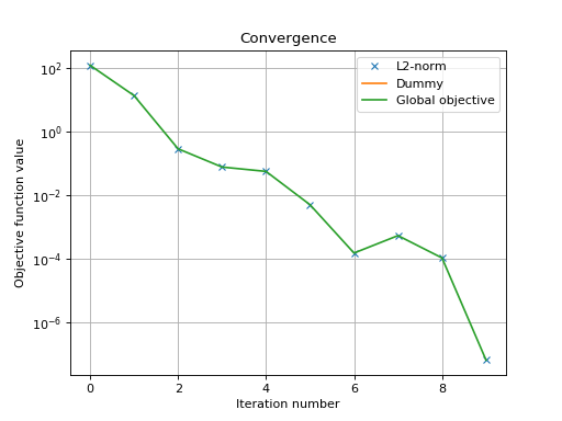
The above graph shows an exponential convergence of the objective function. The global objective is obviously only composed of the L2-norm as the dummy function object was defined to always evaluate to 0 (f2._eval = lambda x: 0).