Image reconstruction (Forward-Backward, Total Variation, L2-norm)
This tutorial presents an image reconstruction problem solved by the Forward-Backward splitting algorithm. The convex optimization problem is the sum of a data fidelity term and a regularization term which expresses a prior on the smoothness of the solution, given by
where \(\|\cdot\|_\text{TV}\) denotes the total variation, y are the measurements, g is a masking operator and \(\tau\) expresses the trade-off between the two terms.
Load an image and convert it to grayscale
>>> import matplotlib.image as mpimg
>>> import numpy as np
>>> try:
...     im_original = mpimg.imread('tutorials/lena.png')
... except:
...     im_original = mpimg.imread('doc/tutorials/lena.png')
>>> im_original = np.dot(im_original[..., :3], [0.299, 0.587, 0.144])
and generate a random masking matrix
>>> np.random.seed(14)  # Reproducible results.
>>> mask = np.random.uniform(size=im_original.shape)
>>> mask = mask > 0.85
which masks 85% of the pixels. The masked image is given by
>>> g = lambda x: mask * x
>>> im_masked = g(im_original)
The prior objective to minimize is defined by
which can be expressed by the toolbox TV-norm function object, instantiated with
>>> from pyunlocbox import functions
>>> f1 = functions.norm_tv(maxit=50, dim=2)
The fidelity objective to minimize is defined by
which can be expressed by the toolbox L2-norm function object, instantiated with
>>> tau = 100
>>> f2 = functions.norm_l2(y=im_masked, A=g, lambda_=tau)
Note
We set \(\tau\) to a large value as we trust our measurements and want the solution to be close to them. For noisy measurements a lower value should be considered.
The step size for optimal convergence is \(\frac{1}{\beta}\) where \(\beta=2\tau\) is the Lipschitz constant of the gradient of \(f_2\) [BT09a]. The Forward-Backward splitting algorithm is instantiated with
>>> from pyunlocbox import solvers
>>> solver = solvers.forward_backward(step=0.5/tau)
and the problem solved with
>>> x0 = np.array(im_masked)  # Make a copy to preserve im_masked.
>>> ret = solvers.solve([f1, f2], x0, solver, maxit=100)
Solution found after 93 iterations:
    objective function f(sol) = 4.268861e+03
    stopping criterion: RTOL
Let’s display the results:
>>> import matplotlib.pyplot as plt
>>> fig = plt.figure(figsize=(8, 2.5))
>>> ax1 = fig.add_subplot(1, 3, 1)
>>> _ = ax1.imshow(im_original, cmap='gray')
>>> _ = ax1.axis('off')
>>> _ = ax1.set_title('Original image')
>>> ax2 = fig.add_subplot(1, 3, 2)
>>> _ = ax2.imshow(im_masked, cmap='gray')
>>> _ = ax2.axis('off')
>>> _ = ax2.set_title('Masked image')
>>> ax3 = fig.add_subplot(1, 3, 3)
>>> _ = ax3.imshow(ret['sol'], cmap='gray')
>>> _ = ax3.axis('off')
>>> _ = ax3.set_title('Reconstructed image')
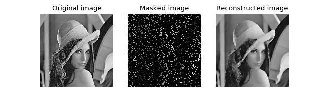
The above figure shows a good reconstruction which is both smooth (the TV prior) and close to the measurements (the L2 fidelity).