Compressed sensing using douglas-rachford

This tutorial presents a compressed sensing problem solved by the douglas-rachford splitting algorithm. The problem can be expressed as follow :

\[\operatorname{arg\,min}\limits_x \|x\|_1 \hspace{1cm} \text{such that} \hspace{1cm} \|Ax-y\|_2 \leq \epsilon\]

where y are the measurements and A is the measurement matrix.

The number of measurements M is computed with respect to the signal size N and the sparsity level K :

>>> N = 5000
>>> K = 100
>>> import numpy as np
>>> M = int(K * max(4, np.ceil(np.log(N))))
>>> print('Number of measurements : %d' % (M,))
Number of measurements : 900
>>> print('Compression ratio : %3.2f' % (float(N)/M,))
Compression ratio : 5.56

Note

With the above defined number of measurements, the algorithm is supposed to very often perform a perfect reconstruction.

We generate a random measurement matrix A :

>>> np.random.seed(1)  # Reproducible results.
>>> A = np.random.standard_normal((M, N))

Create the K sparse signal x :

>>> x = np.zeros(N)
>>> I = np.random.permutation(N)
>>> x[I[0:K]] = np.random.standard_normal(K)
>>> x = x / np.linalg.norm(x)

Generate the measured signal y :

>>> y = np.dot(A, x)

The first objective function to minimize is defined by

\[f_1(x) = \|x\|_1\]

which can be expressed by the toolbox L1-norm function object. It can be instantiated as follow :

>>> from pyunlocbox import functions
>>> f1 = functions.norm_l1()

The second objective function to minimize is defined by

\[f_2(x) = i_S(x)\]

where \(i_S()\) is the indicator function of the set S which is zero if z is in the set and infinite otherwise. The set S is defined by \(\left\{z \in \mathbb{R}^N \mid \|A(z)-y\|_2 \leq \epsilon \right\}\). This function can be expressed by the toolbox L2-ball function object which can be instantiated as follow :

>>> f2 = functions.proj_b2(epsilon=1e-7, y=y, A=A, tight=False,
... nu=np.linalg.norm(A, ord=2)**2)

Now that the two function objects to minimize (the L1-norm and the L2-ball) are instantiated, we can instantiate the solver object. To solve this problem, we use the douglas-rachford splitting algorithm which is instantiated as follow :

>>> from pyunlocbox import solvers
>>> solver = solvers.douglas_rachford(step=1e-2)

After the instantiations of the functions and solver objects, the setting of a starting point x0, the problem is solved by the toolbox solving function as follow :

>>> x0 = np.zeros(N)
>>> ret = solvers.solve([f1, f2], x0, solver, rtol=1e-4, maxit=300)
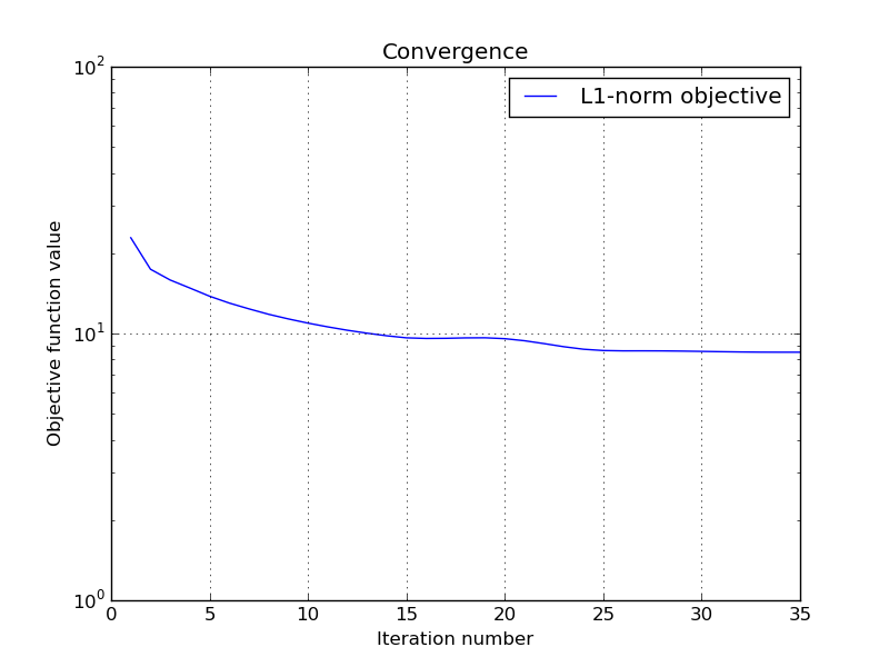
Solution found after 35 iterations :
    objective function f(sol) = 8.508725e+00
    stopping criterion : RTOL

Let’s display the results :

>>> try:
...     import matplotlib, sys
...     cmd_backend = 'matplotlib.use("AGG")'
...     _ = eval(cmd_backend) if 'matplotlib.pyplot' not in sys.modules else 0
...     import matplotlib.pyplot as plt
...     _ = plt.figure()
...     _ = plt.plot(x, 'o', label='Original')
...     _ = plt.plot(ret['sol'], 'xr', label='Reconstructed')
...     _ = plt.grid(True)
...     _ = plt.title('Achieved reconstruction')
...     _ = plt.legend(numpoints=1)
...     _ = plt.xlabel('Signal dimension number')
...     _ = plt.ylabel('Signal value')
...     _ = plt.savefig('doc/tutorials/cs_dr_results.pdf')
...     _ = plt.savefig('doc/tutorials/cs_dr_results.png')
... except:
...     pass

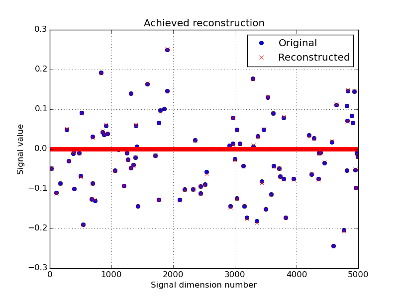
The above figure shows a good reconstruction which is both sparse (thanks to the L1-norm objective) and close to the measurements (thanks to the L2-ball constraint).

Let’s display the convergence of the objective function :

>>> try:
...     objective = np.array(ret['objective'])
...     _ = plt.figure()
...     _ = plt.semilogy(objective[:, 0], label='L1-norm objective')
...     _ = plt.grid(True)
...     _ = plt.title('Convergence')
...     _ = plt.legend()
...     _ = plt.xlabel('Iteration number')
...     _ = plt.ylabel('Objective function value')
...     _ = plt.savefig('doc/tutorials/cs_dr_convergence.pdf')
...     _ = plt.savefig('doc/tutorials/cs_dr_convergence.png')
... except:
...     pass