Compressed sensing using forward-backward

This tutorial presents a compressed sensing problem solved by the forward-backward splitting algorithm. The problem can be expressed as follow :

\[\operatorname{arg\,min}\limits_x ||Ax-y||^2 + \tau ||x||_1\]

where y are the measurements and A is the measurement matrix.

We first declare the signal size N and the sparsity level K :

>>> N = 5000
>>> K = 100

The number of measurements M is computed with respect to the size of the signal N and the sparsity level K :

>>> import numpy as np
>>> R = max(4, np.ceil(np.log(N)))
>>> M = K * R
>>> print('Number of measurements : %d' % (M,))
Number of measurements : 900
>>> print('Compression ratio : %3.2f' % (N/M,))
Compression ratio : 5.56

Note

With the above defined number of measurements, the algorithm is supposed to very often perform a perfect reconstruction.

We now generate a random measurement matrix :

>>> np.random.seed(1)  # Reproducible results.
>>> A = np.random.standard_normal((M, N))

And create the K sparse signal :

>>> x = np.zeros(N)
>>> I = np.random.permutation(N)
>>> x[I[0:K]] = np.random.standard_normal(K)
>>> x = x / np.linalg.norm(x)

We are now able to compute the measured signal :

>>> y = np.dot(A, x)

The first objective function to minimize is defined by :

\[f_1(x) = ||x||_1\]

which is an L1-norm. The L1-norm function object is part of the toolbox standard function objects and can be instantiated as follow (the regularization parameter \(\tau\) is implicitly set to 1.0):

>>> from pyunlocbox import functions
>>> f1 = functions.norm_l1(verbosity='none')

Note

You can also pass a verbosity of 'low' or 'high' if you want some informations about the norm evaluation. Please see the documentation of the norm function object for more information on how to instantiate norm objects (pyunlocbox.functions.norm).

The second objective function to minimize is defined by :

\[f_2(x) = ||Ax-b||_2^2\]

which is an L2-norm that is also part of the standard function objects. It can be instantiated as follow :

>>> f2 = functions.norm_l2(y=y, A=A, verbosity='none')

or alternatively as follow :

>>> A_ = lambda x: np.dot(A, x)
>>> At_ = lambda x: np.dot(np.transpose(A), x)
>>> f3 = functions.norm_l2(y=y, A=A_, At=At_, verbosity='none')

Note

In this case the forward and adjoint operators were passed as real operators not as matrices.

A third alternative would be to define the function object by hand :

>>> f4 = functions.func()
>>> f4.grad = lambda x: 2.0 * np.dot(np.transpose(A), np.dot(A, x) - y)
>>> f4.eval = lambda x: np.linalg.norm(np.dot(A, x) - y)**2

Note

The three alternatives to instantiate the function objects (f2, f3 and f4) are strictly equivalent and will give the exact same results.

Now that the two function objects to minimize (the L1-norm and the L2-norm) are instantiated, we can instantiate the solver object. The step size for optimal convergence is \(\frac{1}{\beta}\) where \(\beta\) is given by

\[\beta = 2 \cdot \operatorname{norm}(A)^2\]

To solve this problem, we use the forward-backward splitting algorithm which is instantiated as follow :

>>> gamma = 0.5 / np.linalg.norm(A, ord=2)**2
>>> from pyunlocbox import solvers
>>> solver = solvers.forward_backward(method='FISTA', gamma=gamma)

Note

See the solver documentation for more information (pyunlocbox.solvers.forward_backward).

The problem is then solved by executing the solver on the objective functions, after the setting of a starting point x0 :

>>> x0 = np.zeros(N)
>>> ret = solvers.solve([f1, f2], x0, solver, relTol=1e-4, maxIter=300)
Solution found after 176 iterations :
    objective function f(sol) = 8.221302e+00
    last relative objective improvement : 8.363264e-05
    stopping criterion : REL_TOL

Note

See the solving function documentation for more information on the parameters and the returned values (pyunlocbox.solvers.forward_backward).

Lets display the results :

>>> import matplotlib, sys
>>> cmd_backend = 'matplotlib.use("AGG")'
>>> _ = eval(cmd_backend) if 'matplotlib.pyplot' not in sys.modules else 0
>>> import matplotlib.pyplot as plt
>>> _ = plt.figure()
>>> _ = plt.plot(x, 'o', label='Original')
>>> _ = plt.plot(ret['sol'], 'xr', label='Reconstructed')
>>> _ = plt.grid(True)
>>> _ = plt.title('Achieved reconstruction')
>>> _ = plt.legend(numpoints=1)
>>> _ = plt.xlabel('Signal dimension number')
>>> _ = plt.ylabel('Signal value')
>>> _ = plt.savefig('doc/tutorials/compressed_sensing_1_results.pdf')
>>> _ = plt.savefig('doc/tutorials/compressed_sensing_1_results.png')

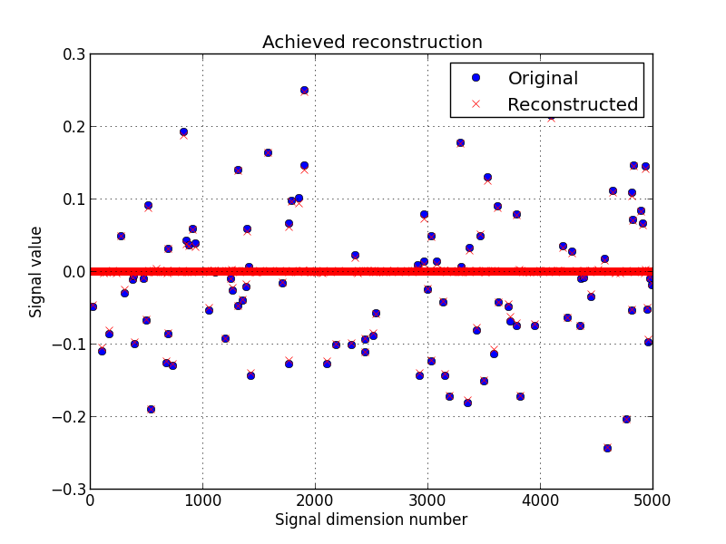
The above figure shows a good reconstruction which is both sparse (thanks to the L1-norm objective) and close to the measurements (thanks to the L2-norm objective).

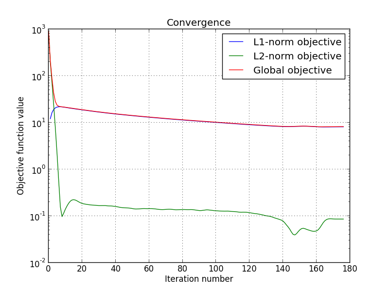
We can also display the convergence of the two objective functions :

>>> objective = np.array(ret['objective'])
>>> _ = plt.figure()
>>> _ = plt.semilogy(objective[:, 0], label='L1-norm objective')
>>> _ = plt.semilogy(objective[:, 1], label='L2-norm objective')
>>> _ = plt.semilogy(np.sum(objective, axis=1), label='Global objective')
>>> _ = plt.grid(True)
>>> _ = plt.title('Convergence')
>>> _ = plt.legend()
>>> _ = plt.xlabel('Iteration number')
>>> _ = plt.ylabel('Objective function value')
>>> _ = plt.savefig('doc/tutorials/compressed_sensing_1_convergence.pdf')
>>> _ = plt.savefig('doc/tutorials/compressed_sensing_1_convergence.png')